1D DCGAN for waveform generation
23 Jun 2021 deep-learningI have a long-term goal of making a GAN that is capable of generating songs similar to the provided training data, mostly as a learning exercise. The idea would be to operate on waveforms directly using convolution, instead of deferring to MIDI approaches.
In the end I imagine I’ll try replicating something like jukebox from OpenAI using VQ-VAE, but for now I’m sticking to DCGAN-like model, except that 1d.
For this article we’ll start a lot smaller and just try to get a GAN to generate a Gaussian curve. The training data will be 10k different 100-sample .wav files that all contain a single centered Gaussian curve with some normal noise. I’m going to be using Pytorch and torchaudio.
The models
Here is what my generator looks like:
class Generator(nn.Module):
    def __init__(self, nz, ngf):
        super(Generator, self).__init__()

        assert(ngf % 32 == 0 and ngf >= 32)

        self.main = nn.Sequential(
            nn.ConvTranspose1d(
                in_channels=nz,
                out_channels=ngf,
                kernel_size=4,
                stride=1,
                padding=0,
                dilation=1,
                bias=False,
            ),
            nn.BatchNorm1d(ngf),
            nn.LeakyReLU(0.2, inplace=True),
            nn.Dropout(p=0.2),

            nn.ConvTranspose1d(
                in_channels=ngf,
                out_channels=ngf // 2,
                kernel_size=4,
                stride=2,
                padding=0,
                dilation=1,
                bias=False,
            ),
            nn.BatchNorm1d(ngf // 2),
            nn.LeakyReLU(0.2, inplace=True),
            nn.Dropout(p=0.2),

            nn.ConvTranspose1d(
                in_channels=ngf // 2,
                out_channels=ngf // 4,
                kernel_size=4,
                stride=2,
                padding=0,
                dilation=1,
                bias=False,
            ),
            nn.BatchNorm1d(ngf // 4),
            nn.LeakyReLU(0.2, inplace=True),
            nn.Dropout(p=0.2),

            nn.ConvTranspose1d(
                in_channels=ngf // 4,
                out_channels=ngf // 8,
                kernel_size=4,
                stride=2,
                padding=0,
                dilation=1,
                bias=False,
            ),
            nn.BatchNorm1d(ngf // 8),
            nn.LeakyReLU(0.2, inplace=True),
            nn.Dropout(p=0.2),

            nn.ConvTranspose1d(
                in_channels=ngf // 8,
                out_channels=1,
                kernel_size=10,
                stride=2,
                padding=0,
                dilation=1,
                bias=False,
            ),
            nn.Tanh(),
        )

    def forward(self, input):
        return self.main(input)
And here is what my discriminator looks like:
class Discriminator(nn.Module):
    def __init__(self, ndf):
        super(Discriminator, self).__init__()

        assert(ndf % 16 == 0 and ndf >= 16)

        self.main = nn.Sequential(
            nn.Conv1d(
                in_channels=1,
                out_channels=(ndf // 16),
                kernel_size=4,
                stride=1,
                padding=0,
                dilation=1,
                bias=False
            ),
            nn.BatchNorm1d(ndf // 16),
            nn.LeakyReLU(0.2, inplace=True),
            nn.Dropout(p=0.2),

            nn.Conv1d(
                in_channels=(ndf // 16),
                out_channels=(ndf // 8),
                kernel_size=4,
                stride=2,
                padding=0,
                dilation=1,
                bias=False
            ),
            nn.BatchNorm1d(ndf // 8),
            nn.LeakyReLU(0.2, inplace=True),
            nn.Dropout(p=0.2),

            nn.Conv1d(
                in_channels=(ndf // 8),
                out_channels=(ndf // 4),
                kernel_size=4,
                stride=2,
                padding=0,
                dilation=1,
                bias=False,
            ),
            nn.BatchNorm1d(ndf // 4),
            nn.LeakyReLU(0.2, inplace=True),
            nn.Dropout(p=0.2),

            nn.Conv1d(
                in_channels=(ndf // 4),
                out_channels=(ndf // 2),
                kernel_size=4,
                stride=2,
                padding=0,
                dilation=1,
                bias=False
            ),
            nn.BatchNorm1d(ndf // 2),
            nn.LeakyReLU(0.2, inplace=True),
            nn.Dropout(p=0.2),

            nn.Conv1d(
                in_channels=(ndf // 2),
                out_channels=ndf,
                kernel_size=4,
                stride=2,
                padding=0,
                dilation=1,
                bias=False
            ),
            nn.BatchNorm1d(ndf),
            nn.LeakyReLU(0.2, inplace=True),
            nn.Dropout(p=0.2),

            nn.Conv1d(
                in_channels=ndf,
                out_channels=1,
                kernel_size=4,
                stride=2,
                padding=0,
                dilation=1,
                bias=False
            ),
        )

    def forward(self, input):
        return self.main(input)
The goal was to maintain the general idea of strided convolutions of the the DCGAN architecture while incorporating some recommendations from other posts and resources like ganhacks. I guess the main differences are:
- LeakyReLU layers to prevent vanishing gradients;
- Dropout to prevent overfitting;
- Removal of the last Sigmoid layer of the discriminator (paired with the usage of nn.BCEWithLogitsLoss() instead of nn.BCELoss()) to better handle mode collapse, as this effectively prevents the discriminator from getting stuck at zero loss.
You may ocasionally see some weird values for kernel_size, stride, padding and dilation, but the performance of the model shouldn’t be too affected by tiny details like these, and these are the easiest buttons to push when trying to match the input/output dimension of the data.
Data loader
Here is what my Dataset look like. Nothing fancy: Just glob all .wav files form a folder.
from pathlib import Path
import torch
import torchaudio
from torch.utils.data import Dataset

def collect_files(folder_root, formats):
    result = []
    for fmt in formats:
        for path in Path(folder_root).rglob('*.' + fmt):
            result.append(str(path))
    return result

class WavDataset(Dataset):
    def __init__(self, root_dir, formats=['wav']):
        self.files = collect_files(root_dir, formats)

    def __len__(self):
        return len(self.files)

    def __getitem__(self, idx):
        waveform, _ = torchaudio.load(self.files[idx])
        return waveform
Main training script
The actual program looks like this:
device = "cpu"
if torch.cuda.is_available():
    device = "cuda"
    torch.cuda.empty_cache()

# Hyperparameters
instance_to_resume = 13
num_epochs = 5000
batch_size = 100
learning_rate = 5e-5
beta1 = 0.9
nz = 100  # Number of values ("features") in the noise supplised to generator
ngf = 512  # Number of generator feature maps (how many channels it will generate for each noise feature)
ndf = 512  # Number of discriminator feature maps

real_label = 1
fake_label = 0
hard_real_labels = torch.full((batch_size,), real_label, dtype=torch.float32, device=device, requires_grad=False)
hard_fake_labels = torch.full((batch_size,), fake_label, dtype=torch.float32, device=device, requires_grad=False)

# Load all of our songs
dataset = WavDataset(os.path.join('D:', 'AI', 'Wavegen', 'data', 'phantom_100'))
num_samples = len(dataset)
print(f"Detected {num_samples} tracks to use")

# Create loader
data_loader = torch.utils.data.DataLoader(
    dataset=dataset,
    batch_size=batch_size,
    shuffle=True
)

# Create models
generator = Generator(nz, ngf).to(device)
discriminator = Discriminator(ndf).to(device)

# Create optimizers
generator_optimizer = torch.optim.Adam(generator.parameters(), lr=learning_rate, betas=(beta1, 0.999))
discriminator_optimizer = torch.optim.Adam(discriminator.parameters(), lr=learning_rate, betas=(beta1, 0.999))

# Create loss function
loss_func = nn.BCEWithLogitsLoss()

# Train
for epoch in range(num_epochs):
    for i, data in enumerate(data_loader):
        actual_batch_size = data.size()[0]
        sample_length = data.size()[2]
        real_batch = data.to(device)

        # Soften labels (probably don't need to do this every batch as the loader shuffles anyway)
        real_labels = torch.randn_like(hard_real_labels) * 0.10 + hard_real_labels
        fake_labels = torch.randn_like(hard_fake_labels) * 0.10 + hard_fake_labels

        # Train generator
        generator_optimizer.zero_grad()
        noise = torch.randn(actual_batch_size, nz, 1, device=device)
        fake_batch = generator(noise)
        fake_output = discriminator(fake_batch).view(-1)
        generator_loss = loss_func(fake_output, real_labels[:actual_batch_size])
        generator_loss.backward()
        generator_optimizer.step()

        # Train discriminator
        discriminator_optimizer.zero_grad()
        real_output = discriminator(real_batch).view(-1)
        fake_output = discriminator(fake_batch.detach()).view(-1)
        real_loss = loss_func(real_output, real_labels[:actual_batch_size])
        fake_loss = loss_func(fake_output, fake_labels[:actual_batch_size])
        discriminator_loss = fake_loss + real_loss
        discriminator_loss.backward()
        discriminator_optimizer.step()

        # Keep statistics
        gen_grad_param_norms = []
        for param in generator.parameters():
            gen_grad_param_norms.append(param.grad.norm())
        mean_gen_grad_norm = torch.tensor(gen_grad_param_norms).mean().item()
        disc_grad_param_norms = []
        for param in discriminator.parameters():
            disc_grad_param_norms.append(param.grad.norm())
        mean_disc_grad_norm = torch.tensor(disc_grad_param_norms).mean().item()
        mean_real_output = real_output.mean().item()
        mean_fake_output = fake_output.mean().item()
        if i % 10 == 0:
            print(f"Epoch [{epoch+1}/{num_epochs}], Batch [{i+1}/{num_samples // batch_size}] loss_g: {generator_loss:.4f}, loss_d: {discriminator_loss:.4f}, mean_real_output: {mean_real_output:.4f}, mean_fake_output: {mean_fake_output:.4f}, mean_gen_grad_norm: {mean_gen_grad_norm:.4f}, mean_disc_grad_norm: {mean_disc_grad_norm:.4f}")
I opted for the Adam optimizer with very slow training rates as these data are only 100-samples long, so it should be quick to train anyway.
We’re using soft labels in order to try and make things a bit more difficult for the Discriminator. The point is that if the discriminator starts getting everything right all the time there will be no gradients to train with, and no progress. On top of that, along with the usage of Dropout layers, soft labels force the discriminator to be more robust.
Note that we run the discriminator on fake_batch twice. As far as I can tell this is actually the right thing to do: When training the generator from generator_loss.backward() we need the errors to flow back from fake_output all the way to generator, so we obviously need to call discriminator(fake_batch). When training the discriminator from discriminator_loss.backward() we also need the errors to flow from fake_loss through the discriminator, but the loss function being used is different, so the errors and gradients at the discriminator will be different. Pytorch really doesn’t seem to allow direct manipulation of the computation graphs (1, 2), so it means we need to run the discriminator again. We can at least detach fake_batch there though, as we don’t care about those errors flowing back up to the generator.
There are entirely different ways to organize a GAN training loop that avoids this double call to discriminator(fake_batch) (check “strategy 2” on this very helpful reference), but the trade-off involves retaining the computational graph (with discriminator_loss.backward(retain_graph=True)) between generator and discriminator training steps, which can lead to higher memory usage. In my case the batch size is the limiting factor in the training process as a whole, so using that approach actually led to a loss of performance.
Results
Let’s look at some results from some successful trainings.
You may have noticed that the training loop prints out some data. Here is how that looks plotted on graphs:
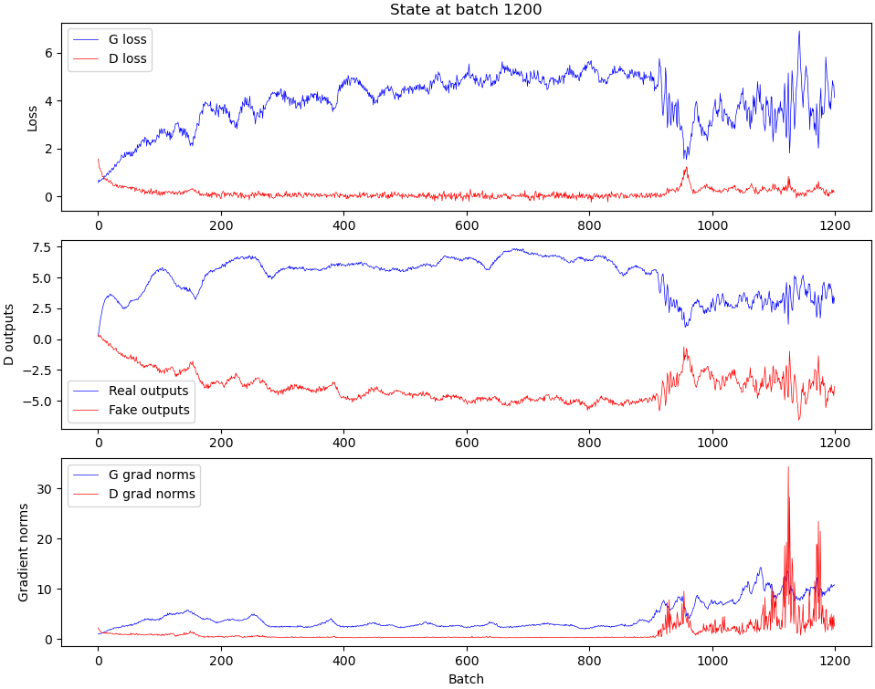
Here’s what these plots mean:
- The topmost plot just shows the generator and discriminator losses;
- The one in the middle shows the average output for the discriminator for real and fake outputs. I’ve opted for classifying based on logits instead of probability values (so as to prevent the discriminator from getting stuck at zero loss), which means that the discriminator should output 1 if it considers a track real, and 0 if it considers it fake, but it is free to output arbitrary values like 100.0 if it really thinks a track is real or -23947.0 if it really really thinks a track is fake. The value of that second plot then describes the mean of these outputs for a given batch;
- The plot on the bottom describes the average magnitude of the gradients for all weights in the generator and discriminator, and is a rough measurement of “how much the weights changed” for a given batch, i.e. “how much it learned.
You may notice that fake_output is basically a rescaled and flipped version of G loss here by the way, but this is just an artifact of our choice of loss functions.
The most interesting aspect of this for me was that I always figured that during the training process I’d see a gradual improvement of my output as time went on. Not once did this happen. There is always a very harsh transition where the model goes from outputting garbage to outputting something most of the way there.
Here is what sample generator outputs (red) look like when compared to the ideal output (blue) during training, at batch 200 and onwards:
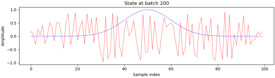
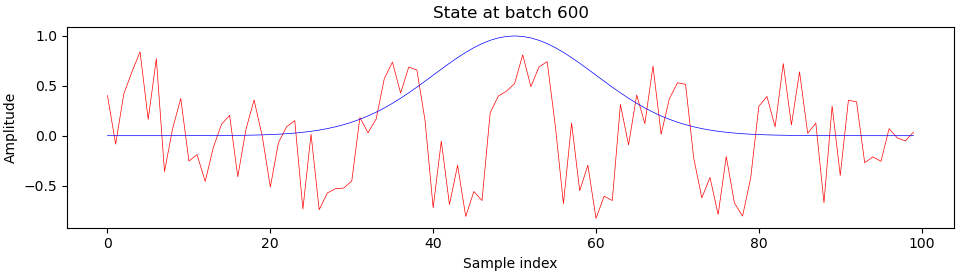
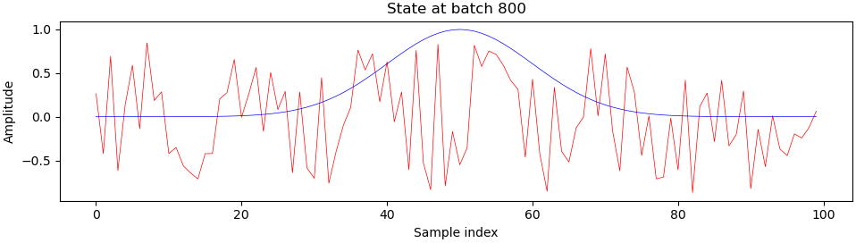
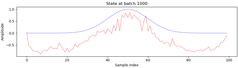
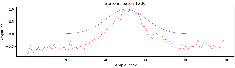
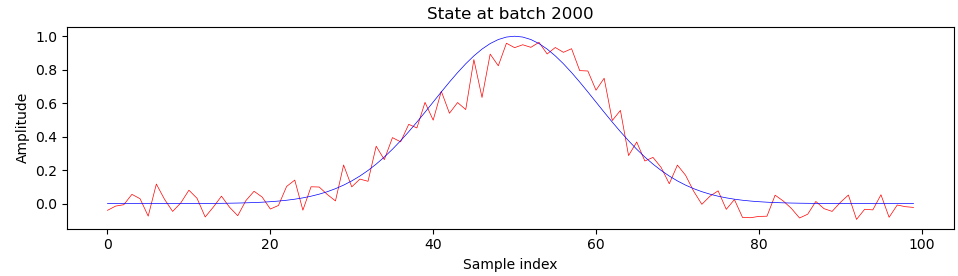
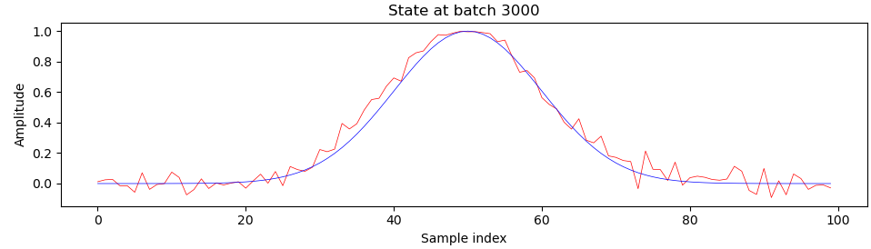
You can see that something really interesting happens right around batch 900, which is right about where we see those harsh transitions on the progress plot. I’m still a beginner at deep learning and GANs, so I’m not entirely sure what exactly, but please let me know if you have any ideas.
Another interesting thing I’ve noticed is that GANs seem to reach a minimum loss at some point, and then progressively diverge, in some ways. Here is an entirely different training process (with all the same parameters) that was left training for way too long:
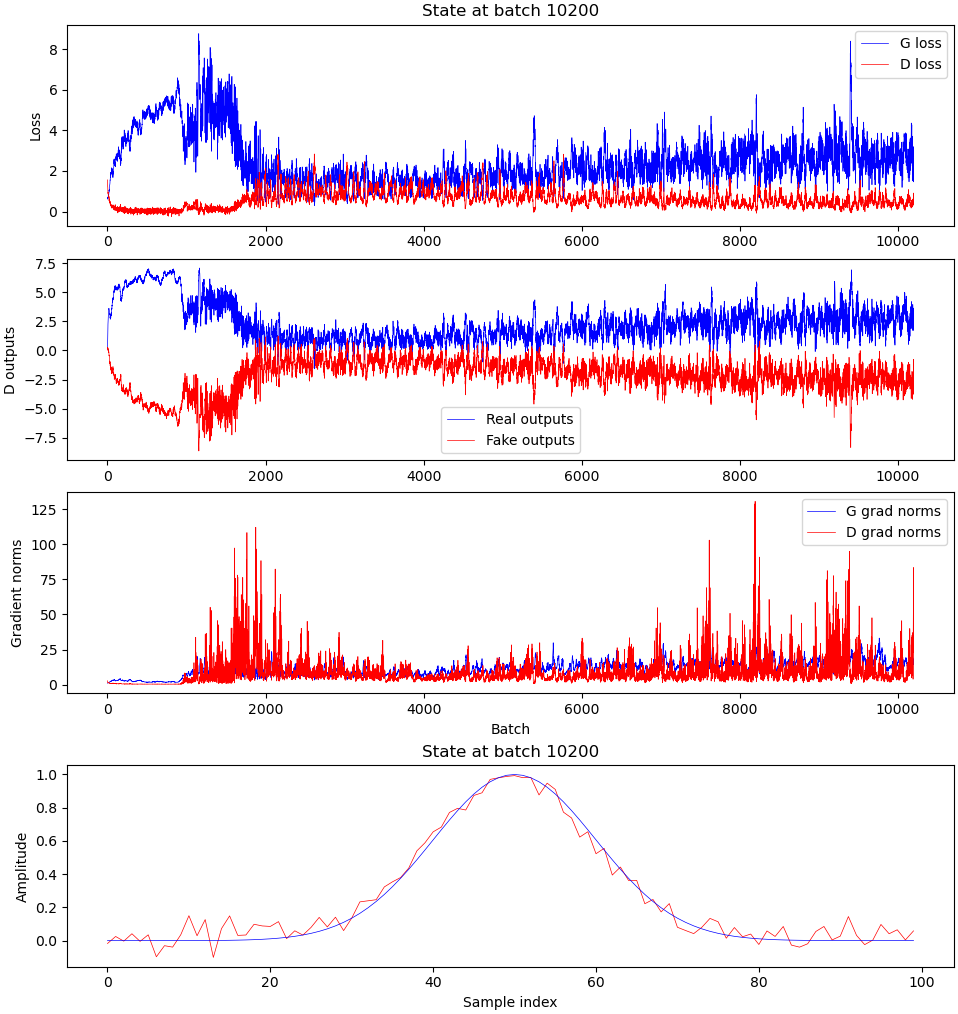
Again, “the transition” happens around batch 900, but you can see that the generator loss tends to slowly increase after having reached a minimum near batch 4000 or so. The discriminator loss tends to decrease over time too, with the average outputs for real and fake samples diverging in score, which is a bad sign: Ideally the discriminator outputs should converge to the same value as the generated samples become more and more similar to the training data, which doesn’t happen here.
Also, as far as I can tell the fact that the norm of generator/discriminator weights also never seem to taper off suggests that it’s either learning too fast or that it’s beginning to overfit the training data.
Conclusion
It was pretty easy to find some references/recommendations on how to write a Pytorch GAN, but I struggled to find references that helped me make sense of the reasoning behind some of those choices, and also had trouble finding references that helped me debug the training process as a whole. Hopefully this post helps in that area, and shows a bit how a GAN training process should feel like.
In future posts I really want to investigate what is happening to these weights during “the transition”, and also measure the impact of some of those choices, like Dropout layers and hyperparameter values, so stay tuned!
References
- https://github.com/soumith/ganhacks
- https://openai.com/blog/jukebox/
- https://pytorch.org/tutorials/beginner/dcgan_faces_tutorial.html
- https://www.fatalerrors.org/a/detach-when-pytorch-trains-gan.html