Pytorch and neural network conventions and notations
17 Dec 2022 deep-learningI’ve been getting into machine learning with Pytorch these past few months, and one of my notes which has gotten the most mileage is this “deconfuser” note where I write out all the useful conventions that I need, but occasionally forget. I figured there’s a chance somebody finds them useful, and it would be a good simple post to get some traction and get back to blogging more.
Here it is:
Conventions
Imagine a neural network with a single 3x4 linear layer:
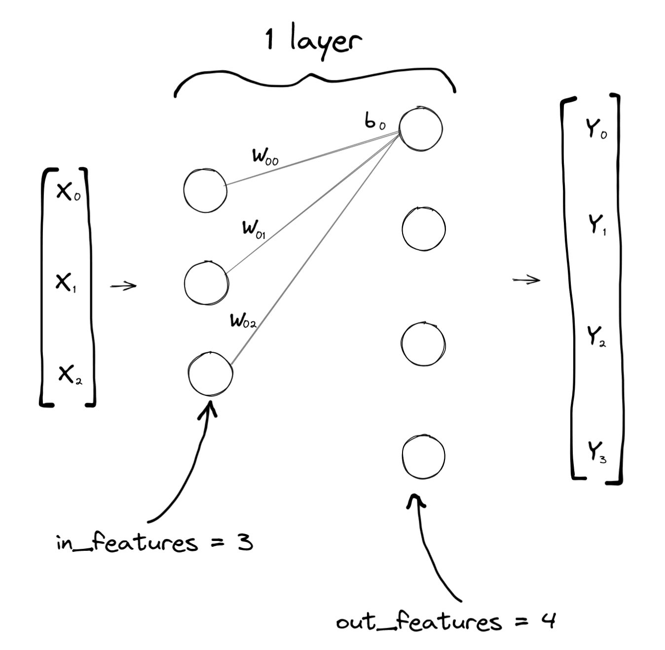
Note that it has two columns of circles (“neurons”), but it is a single layer: Its easier to think of the layer as the thing between the neurons instead of an actual layer of neurons (which would be one of those columns).
You can describe the layer’s weights and biases with matrices W and B like this:
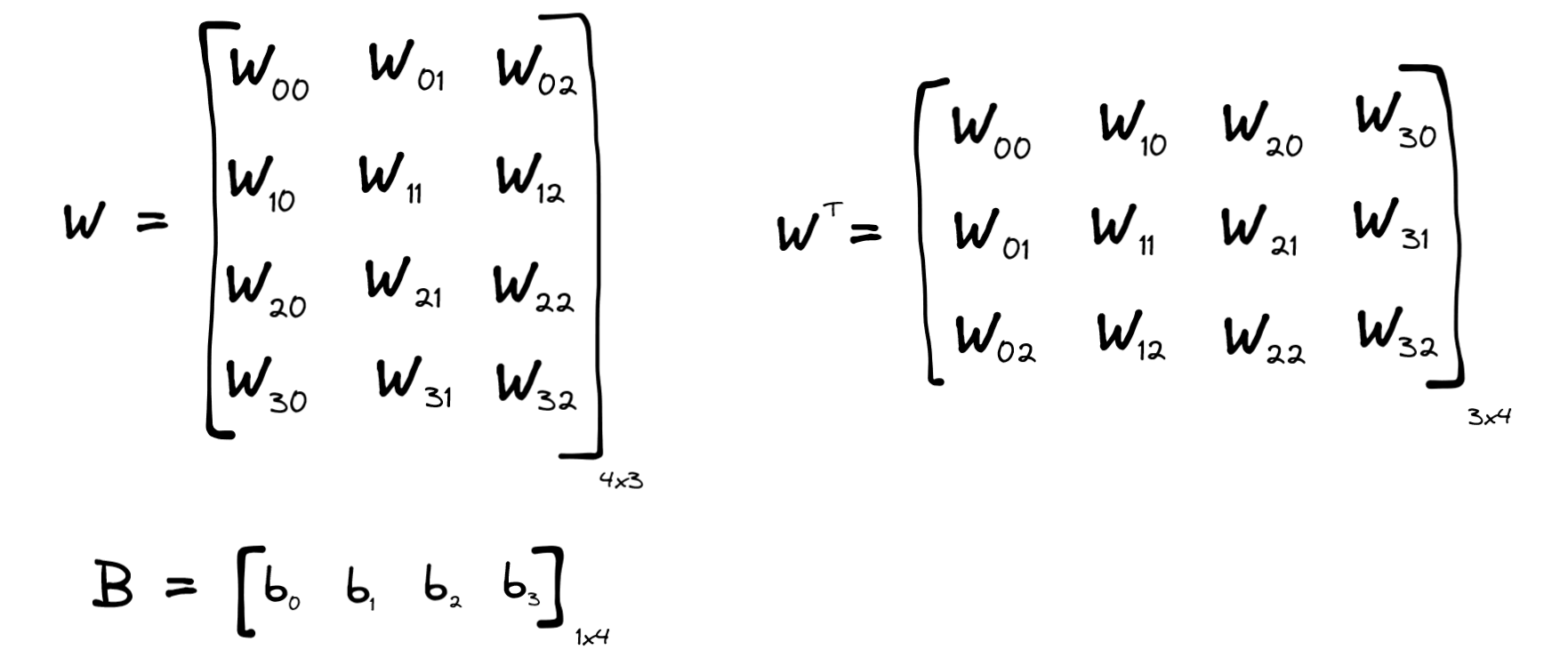
Notice their shapes on the bottom right (number of rows x number of columns). Sometimes you will see W drawn transposed instead, like how I’ve also drawn it on the right in the above image (in this case with 3 rows and 4 columns).
This is how you describe that layer in Pytorch:
import torch

layer = torch.nn.Linear(in_features=3, out_features=4, bias=True)
print(layer.weight.shape)  # Prints [4, 3]
print(layer.bias.shape)    # Prints [4]
Note that it has a 4x3 matrix of weights, which is why I chose to draw W in that way. Also note that technically the bias is a line vector (it has only one dimension with 4 values) instead of being a 1x4 row vector. It’s more useful to think of these as 1xN row vectors instead of line vectors though, for reasons we’ll get to at the Broadcasting section below.
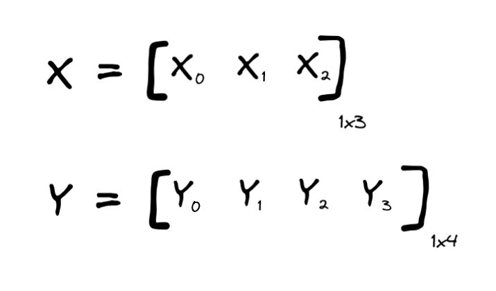
The layer receives a 3-dimensional input X, and produces a 4-dimensional output Y. Again, they’re drawn vertically (kinda like column vectors) on the neural network diagram because it sort of fits, but in Pytorch we’d rather think of them as row vectors.
This is how you apply that layer to a tensor X and receive a tensor Y in Pytorch:
X = torch.rand(3)
layer = torch.nn.Linear(in_features=3, out_features=4, bias=True)

# The generic way of applying any layer
Y = layer(X)

# What torch.nn.Linear does internally
Y_manual = X @ layer.weight.transpose(0, 1) + layer.bias

assert (Y == Y_manual).all().item()  # y and y_manual are the exact same
The @ operator actually just [maps][https://github.com/pytorch/pytorch/blob/6dcc214ac273d594b8a9a30e1f90e30a3c1e40c8/torch/_tensor.py#L885] to [torch.matmul][https://pytorch.org/docs/stable/generated/torch.matmul.html], which is a regular matrix multiply.
The .transpose(0, 1) just transposes the dimensions 0 and 1, so rows with columns. Drawing it out, Y and Y_manual are both computed by the simple linear layer function:
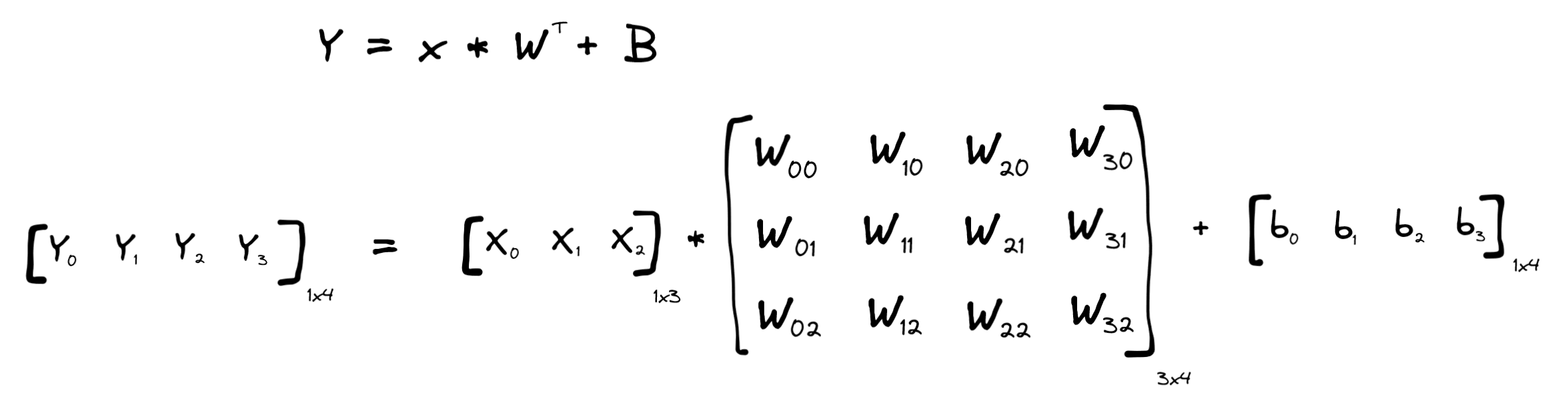
According to the matrix multiply rules, you’ll see you can perform the multiplication of matrices with shapes [1, 3] * [3, 4], (as the two numbers closer together are the same (3)) and that it will lead to a result with shape [1, 4] (the two numbers that are further apart), so that everything works out. Well, except for how X is not really a 1x3 row vector and is really a line vector… I think it’s time:
Broadcasting
I’ve been saying that X, Y and B are row vectors so far, but in Pytorch they’re 1-dimensional line vectors. Who’s to say they don’t represent a column instead of a row?
Well Pytorch has this mechanism called “broadcasting”, where tensors can receive extra dimensions to make their shapes match up with other tensor shapes, in order to be able to perform some operation on them.
For example, look at this:
t1 = torch.tensor([1, 2, 3])                     # Shape [3] <--- line vector
t2 = torch.tensor([[10, 20, 30], [40, 50, 60]])  # Shape [2, 3]  <--- 2D matrix

s = t1 + t2
print(s)         # Prints [[11, 22, 33], [41, 52, 63]]
print(s.shape)   # Prints [2, 3]  <--- 2D matrix
Note that it “broadcast” (here meaning copy-pasted) the t1 tensor values into two identical rows of a “temporary tensor” [[1, 2, 3], [1, 2, 3]] that could then be added with t2 element-wise.
To know if the broadcast mechanism can help your case, you can do this rule of thumb:
- Tensor shapes are aligned to the right:
t2: [2, 3] t1: [3] - Expand the tensor with fewer dimensions to have “1” for all the other dimensions:
t2: [2, 3] t1: [1, 3] - Pytorch will “broadcast” if and only if for each dimension you have an equal number of values (like how we have “3” for the right-most dimension there), or one of the tensors has just 1 value (like how we have 2 and 1 for the left-most dimension there). If one of the tensors has a single value for a dimension, Pytorch will just copy-paste that value until that the two tensors end up with the same number of values for that particular dimension (which is what we saw on the snippet above when we did
s = t1 + t2)
This is why I said 1-dimensional vectors are kind of the same as row-vectors: Pytorch will broadcast them from being [N] to [1, N] before you try performing an operation (like a matrix multiply).
This is why we could do this:
layer = torch.nn.Linear(in_features=3, out_features=4, bias=True)

X = torch.rand(3)                  # Shape    [3]
Wt = layer.weight.transpose(0, 1)  # Shape [3, 4]
B = layer.bias                     # Shape    [4]

Y_manual =        X @ Wt     + B
# Shapes:       [3] @ [3, 4] + [4]
# Shapes:    [1, 3] @ [3, 4] + [4]     (after broadcasting X)
# Shapes:         [1, 4]     + [4]     (after matrix multiply)
# Shapes:         [1, 4]     + [1, 4]  (after broadcasting B)
# Shapes:                [1, 4]        (after adding B)
Batch matrix multiply
There’s one last thing I think still fits in this post: In Pytorch models you rarely have a single 2D matrix for a tensor: You’ll have many more dimensions (batch, channels, etc.). What actually happens if we do something like this?
X = torch.rand((10, 2, 3))  # Shape [10, 2, 3]

# Like before, this has a [3, 4] weight tensor and a [4] bias tensor
layer = torch.nn.Linear(in_features=3, out_features=4, bias=True)

# These are all identical, and end up with shape [10, 2, 4]
Y = layer(X)
Y_manual = X @ layer.weight.transpose(0, 1) + layer.bias
Y_matmul = torch.matmul(X, layer.weight.transpose(0, 1)) + layer.bias
You can think of that 3-dimensional X as being 10 groups of [2, 3] matrices. When you apply layer (or use the @ operator, or call torch.matmul), Pytorch is going to broadcast layer’s weight and biases, and then perform each of the ten [2, 3] * [3, 4] matrix multiplies independently, returning a [10, 2, 4] tensor.
There is also a dedicated [torch.bmm][https://pytorch.org/docs/stable/generated/torch.bmm.html] function for performing the batch matrix multiply. However, annoyingly, this function doesn’t perform broadcasting and only works when the two arguments are tensors with exactly 3 dimensions:
layer = torch.nn.Linear(in_features=3, out_features=4, bias=True)

X   = torch.rand((20, 2, 3))        # Shape [20, 2, 3]
Wt  = layer.weight.transpose(0, 1)  # Shape     [3, 4]
Wte = Wt.expand(20, 3, 4)           # Shape [20, 3, 4]

Y = torch.bmm(X, Wt)                # Raises an error
Y = torch.bmm(X, Wte)               # OK
Finally, what happens if you do a matmul with both tensor arguments having more than 2 dimensions?
A = torch.tensor([  # Shape [2, 2, 3]
    [[1, 2, 3],
     [4, 5, 6]],

    [[7, 8, 9],
     [10, 11, 12]]
])

B = torch.tensor([  # Shape [2, 3, 4]
    [[2, 2, 2, 2],
     [3, 3, 3, 3],
     [4, 4, 4, 4]],

    [[2, 2, 2, 2],
     [3, 3, 3, 3],
     [4, 4, 4, 4]],
])

C = A @ B           # Shape [2, 2, 4]
# C corresponds to torch.tensor([
#    [[ 20,  20,  20,  20]
#     [ 47,  47,  47,  47]],
#
#    [[ 74,  74,  74,  74],
#     [101, 101, 101, 101]]
#])
assert (C[0] == A[0] @ B[0]).all().item()
assert (C[1] == A[1] @ B[1]).all().item()
Like the asserts suggest, it just does 2-dimensional matrix multiplies pairwise for the two arguments, regardless of how many higher dimensions they have. This means you must have exactly the same number of values in each of the higher dimensions though, and something like this wouldn’t work:
A = torch.tensor([  # Shape [2, 2, 3]
    [[1, 2, 3],
     [4, 5, 6]],

    [[7, 8, 9],
     [10, 11, 12]]
])

B_diff = torch.tensor([  # Shape [3, 3, 4]
    [[2, 2, 2, 2],
     [3, 3, 3, 3],
     [4, 4, 4, 4]],

    [[2, 2, 2, 2],
     [3, 3, 3, 3],
     [4, 4, 4, 4]],

    [[2, 2, 2, 2],
     [3, 3, 3, 3],
     [4, 4, 4, 4]],
])
D = A @ B_diff  # Raises an error, since A and B_diff have incompatible shapes
Broadcasting would also help you in this case though, so you could perform this batch matrix multiplication in these cases:
A = torch.rand((2, 2, 3))  # Theses are the shapes of the tensors
B = torch.rand((2, 3, 4))
C = A @ B  # Ok

A = torch.rand((2, 2, 3))
B = torch.rand(   (3, 4))
C = A @ B  # Ok

A = torch.rand((2, 2, 3))
B = torch.rand((1, 3, 4))
C = A @ B  # Ok

A = torch.rand((1, 2, 2, 3))
B = torch.rand(   (1, 3, 4))
C = A @ B  # Ok

A = torch.rand((1, 2, 2, 3))
B = torch.rand((4, 1, 3, 4))
C = A @ B  # Ok

A = torch.rand((2, 2, 2, 3))
B = torch.rand((4, 1, 3, 4))
C = A @ B  # Error

A = torch.rand((1, 2, 2, 3))
B = torch.rand(   (4, 3, 4))
C = A @ B  # Error

A = torch.rand((1, 2, 2, 3))
B = torch.rand(      (3, 4))
C = A @ B  # Ok
That’s about as much as I wanted to cover on this one. Some of these things always confused me, like how you specify a linear layer like torch.nn.Linear(3, 4) and it actually has a 4x3 weights matrix, but transposes it for the multiply.
I deliberately chose different numbers of values in all dimensions, but if you have square matrices (more often than not) you can see how this can lead to subtle issues and confusion.
Thanks for reading!